Asset allocation is the term used traditionally to describe the apportionment of one's financial assets among the three major asset classes -- cash, bonds, and common stocks. In more recent times, the universe of assets among which an asset allocator might allocate a portfolio has come to include a multitude of other products that the investment and insurance communities have created and marketed.

It is my impression that many financial planners approach asset allocation much as some might approach a buffet dinner. If an item is on the table, they should have some, irrespective of whether or not it is good for them, the faith, perhaps, being that, if it were not good for them, it would not be on the table.

It is, then, not uncommon to encounter elaborately and expensively tailored financial plans that include -- in addition to common stocks, bonds, and cash -- mutual funds, deferred annuities, real estate investment trusts, convertible bonds, preferred stocks, limited partnerships, foreign securities, precious metals, and a multitude of other more complex investment vehicles. There is also computer software which, somehow, will tell us to what extent our portfolio should be deployed in each of these areas.

Outside of stocks, bonds, and cash, it is usually pretty easy to demonstrate that the ownership of any other investment vehicle to achieve legitimate investment objectives, no matter what these objectives may be, is both unnecessary and inefficient.  It is the purpose of this paper to demonstrate further that even the time-honored bond probably falls into this category of investment vehicles that are both unnecessary and inefficient, irrespective of one's investment objectives.

All investing involves trade-offs. If we acquire Investment #1 for a benefit we want, as opposed to Investment #2 that lacks the benefit, it is an absolute certainty that we are sacrificing some other advantage present in Investment #2 that is not present in Investment #1 -- whether we are aware of it or not. If the benefit of Investment #1 that we are receiving is of greater value to us than the benefit of Investment #2 that we are sacrificing, Investment #1 is, of course, the more suitable investment for us. One may, for example, legitimately invest his cash in bank certificates of deposit, instead of U. S. Treasury bills, because he considers the psychic satisfaction of dealing with his local bank a greater benefit than the state income tax exemption on the income earned on U. S. Treasury bills.

By far the most important trade-off in investing, however, is what is known as the risk-reward trade-off. If we expose our capital to greater risk, over time and in the aggregate, we are supposed to reap greater monetary benefits.

The monetary benefits in investing are pretty simple to understand and to measure. They come in the form of interest, dividends, and capital appreciation (or depreciation) and are expressed as rates of total return. Risks, however, are a bit more complicated, both to understand and to measure.

The terms "risk" and "volatility" tend to be used interchangeably. I believe this is semantically unfortunate because the term "risk" implies the possibility of a permanent loss, while the term "volatility" implies that any consequent loss need be only temporary. Understandably, most people are far less uncomfortable contemplating a temporary depreciation in the value of their assets than they are contemplating an outright and irrecoverable loss of those assets.

While volatility is an attribute of an investment, risk is an attribute of both an investment and its owner. An investment that may entail considerable risk for me may entail minimal risk for you. The second variable that needs to be combined with the volatility of an investment to assess its risk to its owner is the owner's "holding period." If the owner's holding period is too short, a given level of volatility may pose for him a great risk; if, on the other hand, his holding period is relatively long, that same level of volatility may pose for him minimal risk.

In the case of a class of investments which fluctuate in value, then, the risk (the probability and magnitude of any permanent loss) is a function both of the nature of the investment and the length of the owner's holding period.

In an effort to quantify all three dimensions of risk -- (1) probability of loss, (2) magnitude of possible loss, and (3) individual holding periods -- mathematicians utilize a concept known as "standard deviation." With respect to rates of return, standard deviation is a measure of the frequency and degree by which the return on an investment varies from its average rate over some period of time -- usually one year.

The very definition of "standard deviation" introduces a second semantic difficulty. Standard deviation interprets returns which "vary" above the average as equal in significance to returns that "vary" below the average. As Mark Twain once remarked, however, "A wife does not so much object to her husband's gambling. She mostly objects to his losing." Standard deviation, which may be described as the mathematical measure of the probable pain in the ownership of an investment, draws no distinction between above-average profits and above-average losses, yet it is only the latter that cause pain.

A good way to try to understand standard deviation is with some examples: The average return on common stocks over the past seventy years has been about 10% per year, with a standard deviation of 20%. This means that, in very close to two-thirds (68%) of those seventy years, the rates of return on common stocks ranged from between 30% (10% plus 20%) to -10% (10% minus 20%). In one-third of those years, the returns were either greater than +30% or less than -10%.

Similarly, for small capitalization stocks, over the past seventy years, the average rate of return has been about 12% per year, with a standard deviation of about 35% per year. The range of returns in two-thirds of those seventy years, then, has been between +47% (12% + 35%) and -23% (12% - 35%). In one-third of those years, the returns were either greater than +47% or less than -23%.

Over long spans of time, the correlation between the rates of return and the standard deviations of asset classes and market sectors has been extremely good. In general, the higher the standard deviation of returns on an asset class, a market, a market sector, or an investment vehicle, the higher has been the rate of return on that particular investment category.

In structuring our portfolio of financial assets, the most critical question we have to address is what degree of volatility in the income on, and value of, our assets we are willing to tolerate. The greater the volatility we are willing to endure, the greater the return, over time, we should expect to earn on our money. Similarly, our tolerance for volatility should be enhanced as we increase the length of our intended holding period for the investment or class of investments being evaluated. And, as noted above, in spite of its shortcomings, the best measure we have, and the universally accepted measure of volatility is standard deviation.

In one of our previous examples, we said that, over the past seventy years, common stocks have delivered an average rate of total return of about 10% per year with a standard deviation of about 20% per year. If we use this data to look forward, we might say that, on average, in two years out of three, we should expect a return on our common stocks that lies between -10% and +30%; while, in the other year, we should expect a return that is either greater than 30% or less than -10%.

Notice, here, that both total return and standard deviation are annualized. The unit of time, or holding period, is one year. If we want to assess the probability of a big gain or a big loss over some longer (or shorter) period of time, we may use the following formula:

Note: For the mathematical perfectionist the following more complex formula is the more precise in that it allows for annual compounding, while the simpler formula above does not:

If, for example, we want to calculate the standard deviation of investing in stocks over a five-year holding period, we simply divide the standard deviation for one year by the square root of five (about 2.2) as follows:

This means that, if our expected holding period is five years, the range of our expected average returns in two-thirds of such five-year holding periods should be within the range of +19% per year (10% plus 9%) and +1% (10% minus 9%). In two-thirds of all five-year holding periods, we should earn less than 19% per year but more than 1% per year; and, in the other-third of all those five-year holding periods, we should earn more than 19% or less than 1% per year.

In the following table, I have reproduced the average annual rates of total return and standard deviations for cash, bonds, and common stocks over various periods from five to seventy years. The figures are calculated from the seventy years of data found in the publication, Stocks, Bonds, Bills, and Inflation 1996 Yearbook, published by Ibbotson Associates -- the most widely used source of data for studies such as this. The proxies for cash, bonds, and stocks used here are 30-day U. S. Treasury bills, 20-year U. S. Government bonds, and the Standard & Poor's Composite Stock Index, respectively.

As the first row of data in the foregoing table indicates, over the past seventy years, the average annual total return on U. S. Government bonds has been 5.2% per year, while the standard deviation for these bonds over the period has been 9.2% per year. This means that, in one-third of these seventy years, the rate of return on U. S. Government bonds has been either greater than 14.4% (5.2% plus 9.2%) or less than -4.0% (5.2% minus 9.2%). How, one might ask, does one earn a negative rate of return on a U. S. Government bond?

The explanation as to how the total returns on a U. S. Government bond can be so volatile, and so frequently negative, is that the price of any bond fluctuates with interest rates. When interest rates go way down, the value of a long-term bond goes way up; and, when interest rates go way up, the value of a long-term bond goes way down. Total return is the sum of the interest payments plus appreciation or minus depreciation. If the deprecation of the value of a bond exceeds its interest payments in a given year, the total return for that year will be negative, just as it would be negative for a stock in a year when its value declined by an amount that exceeded its dividend payments.

Though it received far less publicity, prior to the stock market crash of October 1987, the bond market had crashed in April of 1987. In spite of the stock market crash in that year, however, the average common stock holder enjoyed a net gain in 1987, while the average long-term bond holder experienced a net loss in that year. It is, then, the high volatility of their prices, caused by the high volatility of interest rates, that makes the total returns on long-term bonds so volatile.

The basis for arguing that bonds are both unnecessary and inefficient in an investment portfolio is the observation that, at least over the past seventy years, it has been possible historically to construct a portfolio out of common stocks and cash that has had (1) the same return as a bond portfolio but less risk (volatility as measured by standard deviation), (2) the same risk as a bond portfolio but a greater return, or (3) both a greater return and less risk than that of a bond portfolio. I call these synthetically constructed bonds "barbell bonds," made up of varying proportions of cash on one end and stocks on the other.

A set of computations demonstrating how it has been possible, by blending cash and stocks, to equal the returns on U. S. Government bonds, with less portfolio risk than holding bonds, appears in the following table:

The most dramatic example we note in the foregoing table is that, over the past half century, it has been possible, with a portfolio that was 93% in cash and only 7% in stocks, to match the total return on U. S. Government bonds but with only 39% as much risk as with holding only U. S. Government bonds.

The following table uses the same data, but assumes that portfolios of cash and stocks are created which duplicate the risks (standard deviations) as in the bond portfolios.

Again, the record of the past half-century provides the most dramatic example. A portfolio that was 46% cash and 54% stocks was no more volatile than a portfolio of all U. S. Government bonds, yet it produced an average annual return that was 64% greater than that produced by the all-bond portfolio.

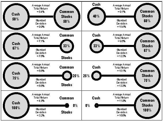
Some pictorial examples of barbell portfolios appear in the following table. As the basis for evaluating risk-return trade-offs in these several cash-stock portfolios, I have used the foregoing Ibbotson-derived data for the half-century following the end of World War II (1946-1995).

The Traditional Barbell Concept in Bond Investing

The concept of barbell investing with cash and common stocks is borrowed from a common practice in the management of bond portfolios. For bond investors who do not wish to undertake the impossible task of predicting interest rate moves, there are two approaches to designing and maintaining a bond portfolio.

One approach is to "ladder" the maturities of one's bonds. One may start by assembling a portfolio with equal amounts of bonds maturing in each year, one through twenty. Then, each year, as bonds mature, they are rolled over into new twenty-year bonds. With such a program, one has an average ten-year maturity portfolio. Half the bonds mature over the first ten years and half mature over the second ten years.

The second approach is a barbell approach. Here the portfolio consists of half cash and half twenty-year bonds. Again, the average maturity of the portfolio is ten years, but it has two other positive attributes. First, it is more liquid, because half the portfolio is already in cash and so does not need to be converted to cash, if and when cash is needed or desired; and, second, studies similar to this one examining bond portfolios indicate that the average return, over time, is actually higher with the barbell bond portfolio than with the laddered bond portfolio with the same average maturity.

Ironically, it would actually have been easier to have implemented barbell bond portfolios made up of cash and stocks and produced the results previously described than it would have been to implement the U. S. Government bond portfolios and have produced the results indicated with them.

Because they are more volatile, the returns on long-term bonds are greater than the returns on short-term bonds. As a long-term bond approaches maturity, however, it becomes a short-term bond. When it is very close to maturity, its return is no greater than the return on cash. The foregoing models for bonds, then, assume that one purchases a twenty-year U. S. Government bond (or a portfolio of such bonds) each year, sells all his bonds after one year (at which time they have become 19-year bonds), and replaces them with new 20-year bonds. Such a high degree of turnover in a bond portfolio would, of course, be expensive and so detract considerably from the overall return. Anybody who owns bonds is faced with exactly this dilemma, however -- whether to hold the bonds until maturity and so reap the lesser rewards of shorter-term bonds through most of the life of the bonds, or to incur the incremental costs of periodically rolling the shortened, but far-from-matured, bonds over into longer, higher-yielding bonds.

In contrast, the owner of the barbell cash and stock portfolio has no such problem. He may achieve his return on cash by simply holding his cash in a bank savings account, and he can achieve his return on stocks by simply assembling and holding a diversified list of common stocks. Neither savings accounts nor common stocks have dates of maturity. Admittedly, he may seek to augment the return on his stock portfolio by buying and selling stocks occasionally, but the foregoing studies are not based upon his actively managing his stock portfolio. Much to the contrary, these results are based upon his buying and holding a representative portfolio, without any sales or repurchases, throughout the assumed holding period -- whether that period is five years, fifty years, or seventy years. If, by giving the stock sector of his portfolio some tender love and care, he can improve his results, relative to the "buy-and-hold" strategy assumed in using a common stock index as a measure of performance, he should be even further ahead of the game.

As acknowledged in an earlier paragraph, all investing involves trade-offs. Do "barbell" bonds offer a free lunch? Our theory says, no. What, then, is that less obvious benefit we forego, relative to a bona fide bond portfolio, when we create a barbell portfolio with both less risk and a greater return?

The answer, of course, is that U. S. Government bonds bestow virtually all their net rewards in the form of periodic interest payments which they disburse to us most religiously every six months. Bonds offer us a built-in plan for systematic cash withdrawals.

In contrast, most of the benefits in common stock investing come in the form of capital appreciation and, if one wants to tap into this capital appreciation income to meet living expenses, he needs to set up his own program of periodic cash withdrawals.

To enjoy the greater returns and/or lesser risks of barbell investing, as opposed to bond investing, one must overcome two psychological hurdles: First, he must ignore the distinction between interest or dividend income and capital appreciation income in measuring the performance of his investments; that is, he must focus solely on "total return" which combines both kinds of income into one number. Second, to the extent that he wants to utilize his assets for living expenses, he must be willing to spend his capital gains income as readily as he spends his interest and dividend income.

History shows us that, by using the barbell approach to asset allocation, whereby a combination of common stocks and cash has been substituted for bonds, one has not had to make sacrifices in either the reliability or the magnitude of his returns; he has, at most, had only to incur an inconvenience in the way he tapped into these returns. For those willing to subject themselves to this inconvenience, however, the rewards have, indeed, been very great.

The purpose of the foregoing discussion has been to reemphasize our conviction that the most successful investing is simple investing. In spite of the myriad of investment products and services available, the most suitable and rewarding portfolios for most investors can probably be created simply by blending cash and common stocks to produce a level of overall portfolio volatility as great as, but no greater than, its owner can comfortably tolerate.

In short, we probably need not and, in fact, probably ought not, look any farther than to cash and common stocks for the ingredients out of which to construct our entire investment portfolio. This, then, is the "how and why" of what we call our "barbell" approach to asset allocation.

Clifford G. Dow
Chartered Financial Analyst
Chartered Financial Consultant

Copyright © 1998 Dow Publishing Company, Inc. All Rights Reserved.

Securities offered through Delta Equity Services Corp. 579 Main St, Bolton MA 01740 800-649-3883. Member NASD MSRB SIPC. Advisory services offered through Delta Global Asset Management, an SEC Registered Investment Advisor and affiliate of Delta Equity Services Corp.